In this series, we’ve introduced vector symbolic architectures (VSAs) and the operations which allow them to robustly and efficiently represent complex structures such as graphs. However, in all the examples we’ve explored so far, we’ve started out by defining our problem in terms of symbols. In other words, we haven’t used any ‘real-world’ data such as images as the input for a vector-symbolic computation. In this tutorial, we’ll explore how to accomplish this and how neural networks can play a role in this process.

Real-World Computation

In this tutorial, we’ll demonstrate a relatively basic example of how neural networks can be integrated with vector-symbolic computation. A common set of images, “Fashion-MNIST,” will be used as our real-world dataset. Each example in the set consists of a picture of an article of clothing accompanied by a class identifier (e.g. “T-shirt”). We’ll start by loading this dataset using the tensorflow-datasets backend:

import tensorflow as tf
import tensorflow_datasets as tfds

import numpy as np
import matplotlib.pyplot as plt

from tqdm import tqdm

#disable TF access to the GPU, it's only being used to load the dataset
tf.config.set_visible_devices([], 'GPU')

dataset_name = "fashion_mnist"
batch_size = 128

#function to load the given dataset in three portions: iterator for training, full
# set of images, and full set of labels

def load_dataset(dataset_name: str,
                split: str,
                *,
                is_training: bool,
                batch_size: int,
                repeat: bool = True):

    #load a batched copy of the dataset
    ds = tfds.load(dataset_name, data_dir="~/data", split=split).cache()
    if repeat:
        ds = ds.repeat()
    if is_training:
        ds = ds.shuffle(10 * batch_size, seed=0)
    ds = ds.batch(batch_size)

    #load full copies of the dataset images and labels
    x_full, y_full = tfds.as_numpy(tfds.load(dataset_name, 
                    split=[split], 
                    data_dir="~/data",
                    shuffle_files=True,
                    as_supervised=True,
                    batch_size=-1,
                    with_info=False))[0]

    return iter(tfds.as_numpy(ds)), x_full, y_full

label_map = {0: "T-Shirt",
             1: "Trouser",
             2: "Pullover",
             3: "Dress", 
             4: "Coat",
             5: "Sandal",
             6: "Shirt",
             7: "Sneaker",
             8: "Bag",
             9: "Ankle Boot",
             }

#load an interator over the dataset and a full copy of it
dataset_train, images_full, labels_full = load_dataset(dataset_name, "train", is_training = True, batch_size = batch_size)

Now that we’ve loaded our dataset, we can inspect it. Here we have an example image:

plt.figure(dpi=100)
plt.imshow(images_full[0,:,:,0], cmap="gray")
print("Image is of a " + label_map[labels_full[0]])

Image is of a Pullover

png

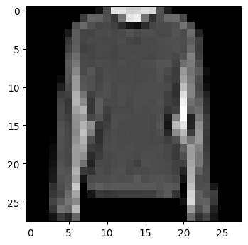
This image is encoded as a single frame of 28 by 28 unsigned, 8-bit integers:

print("Image shape is", images_full[0,...].shape, "and has datatype", images_full.dtype)

Image shape is (28, 28, 1) and has datatype uint8

Vector-Symbolic Classification

One of the most common image processing tasks is image classification. Given an image like we have above, the task is to predict what class the image belongs to. In this case, given a picture of an article of clothing, we would like to be able to predict what it is: a t-shirt, shoe, etc. While trivial for humans, before the advent of modern neural networks this task remained highly challening for computers.

There are hundreds of tutorials which will demonstrate how to use a neural network to classify an image, but in this one we will take a slightly different approach. Instead of using a neural network to transform an input image into a set of class predictions, we will use the network to transform the image into a vector-symbol. Each symbol produced from an image will then be compared to a series of symbols representing each class. The class with the highest similarity to the symbol produced from the image is then the predicted class.

# import JAX which will be used as the backend for the neural network and vector-symbols
import jax.numpy as jnp
from jax import random, vmap, jit, nn, grad

# import the VSA functions we've explicitly defined in the previous notebooks
!git clone https://github.com/wilkieolin/FHRR
from FHRR.fhrr_vsa import *

#install and import the ML libraries for JAX
!pip install optax==0.0.9
!pip install dm-haiku==0.0.5
import haiku as hk
import optax

First, we’ll define a series of symbols which will represent each class of clothing:

key = random.PRNGKey(42)
key, subkey = random.split(key)
#set the dimensionality of the VSA
VSA_dimensionality = 1024
#generate the symbols used to represent each class of clothing
class_codebook = generate_symbols(subkey, len(label_map.keys()), VSA_dimensionality)

#declare a separate instance of each symbol which we can use later
tshirt = class_codebook[0:1,:]
trouser = class_codebook[1:2,:]
pullover = class_codebook[2:3,:]
dress = class_codebook[3:4,:]
coat = class_codebook[4:5,:]
sandal = class_codebook[5:6,:]
shirt = class_codebook[6:7,:]
sneaker = class_codebook[7:8,:]
bag = class_codebook[8:9,:]
ankle_boot = class_codebook[9:,:]

The task the neural network now needs to accomplish is given an input image - a series of 784 8-bit integers - it needs to map it into a vector-symbol. In this case, as we’re still using the Fourier Holographic Reduced Representation, this will be a series of radian-normalized angles - by default, we’ll use 1024 angles in the series (defined by VSA_dimensionality above).

We’ll use a simple neural network with 3 layers to accomplish this mapping between domains. It consists of 12 3x3 convolutional kernels, a 100-neuron fully-connected layer, and a 1024-neuron output. We apply a softsign to the final layer, producing an output which matches the domain of our vector-symbols ([-1, 1]).

#convert 8-bit [0,255] images to [0,1] floating points
def scale_mnist(images):
    return jnp.divide(images, 255)

#use a simple convolutional network
def network_fn(images):
    mlp = hk.Sequential([
                        #layer 1, 12 x (3x3) convolution
                        scale_mnist,
                        hk.Conv2D(12, (3,3)),
                        nn.relu,
                        hk.Flatten(),
                         
                        #layer 2, 100 FC neurons
                        hk.Linear(100),
                        nn.relu,
                         
                        #layer 3, output to a VSA symbol by FC layer
                        hk.Linear(VSA_dimensionality),
                        nn.soft_sign,
    ])

    return mlp(images)

Now, we’ll use Haiku to produce a function we can call to execute this network and initialize a set of parameters for it. In contrast to PyTorch and Tensorflow, here the network is purely functional instead of a stateful object, which leads to some differences in how we’ll train and execute it below.

#return a pure function from the network
network_full = hk.transform(network_fn)
#exclude the rng parameter from the function since it's not used in the model
network = hk.without_apply_rng(network_full)

#generate a new random key
key, subkey = random.split(key)
#use it to initialize the parameters to be used with the network function
params = network.init(subkey, images_full[0:batch_size,...])

Now, we can test our network with the initial, random parameters and inspect the outputs. Just as we designed it, each input image leads to an output which can be considered a vector-symbol. For each output, we can compare it to the symbols we defined and see if they have any similarity:

#produce a series of example outputs from the network
symbols_0 = network.apply(params, images_full[0:batch_size,...])

initial_similarity = similarity_outer(symbols_0, class_codebook)

def plot_similarity(image_symbols, 
                    label_symbols = class_codebook, 
                    classes = list(label_map.values())):
  
    s = similarity_outer(image_symbols, class_codebook)

    plt.figure(dpi=100)
    plt.pcolor(s, vmin=-1, vmax=1, cmap="bwr")
    plt.colorbar()
    plt.xlabel("Class Symbol")
    plt.xticks(jnp.arange(0,10)+0.5, list(label_map.values()), rotation=90)
    plt.ylabel("Input Image")
    plt.title("Similarity Between Image Symbols and Label Symbols")

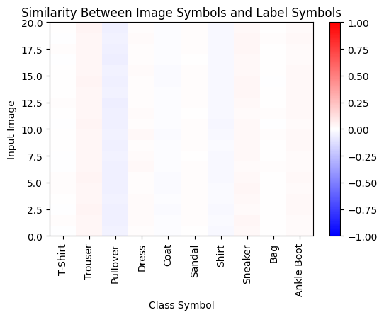
As we can see below, none of the symbols produced from an image by applying the neural network are similar to the symbols in the codebook which define each of the clothing classes. This is what we’d expect, given that random symbols in a VSA are dissimilar, and our neural network has been initialized with random parameters.

plot_similarity(symbols_0[0:20,...])

png

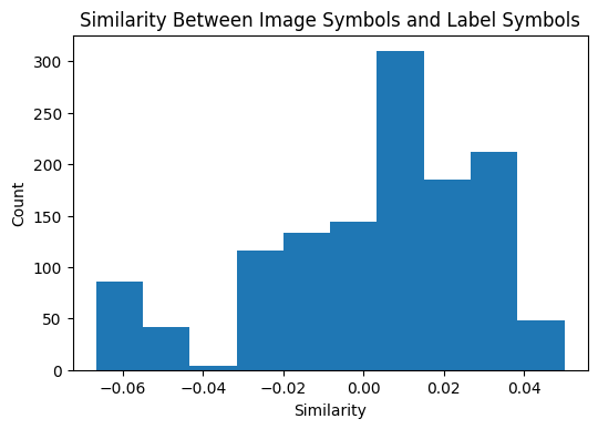
plt.figure(dpi=100)
plt.hist(jnp.ravel(initial_similarity))
plt.xlabel("Similarity")
plt.ylabel("Count")
plt.title("Similarity Between Image Symbols and Label Symbols")

Text(0.5, 1.0, 'Similarity Between Image Symbols and Label Symbols')

png

Training

Now, our task is to figure out how to train the neural network to produce the mapping we want: given an input image of a T-shirt, we want the neural network to produce a symbol which is highly similar to the tshirt symbol. To do this, we’ll define our loss function for the network:

#Calculate the similarity between each symbol and its matching class symbol, then
# invert it and add to one to calculate loss

@jit
def similarity_loss(symbols, labels, class_codebook = class_codebook):
    #for each input symbol, find the matching class symbol based on its label
    one_hot = nn.one_hot(labels, class_codebook.shape[0])
    label_symbols = jnp.matmul(one_hot, class_codebook)
    #calculate the similarity between each symbol produced from an image and its class symbol
    # and subtract it from one to produce a loss we want to minimize
    losses = 1 - similarity(symbols, label_symbols)
    #return the mean loss over each symbol
    loss = jnp.mean(losses)

    return loss

We can call this loss function on the initial batch of image-generated symbols we just produced. Given that as we just observed these symbols are not similar to any class labels, the average loss value is very close to 1.0:

similarity_loss(symbols_0, labels_full[0:batch_size]).item()

0.999203622341156

Now, given that we have a loss function and a neural network, we can use the standard techniques of backpropagation and gradient descent to attempt to train our network. We’ll first create an instance of a standard optimizer:

#declare an instance of the RMSprop optimizer
optimizer = optax.rmsprop(0.001)
#initialize the optimizer
opt_state = optimizer.init(params)

Next, we’ll define a function to calculate loss given a batch of input data, our network, and its current parameters:

#create a function to evaluate loss given the network, parameters, and training batch
def loss_fn(net, params, batch):
    images = batch['image']
    labels = batch['label']
    yhat = net.apply(params, images)

    loss = similarity_loss(yhat, labels)
    return loss

And finally, we’ll use that function to define the update step for our training process. Given the network function, its current parameters, the optimizer, its current parameters, and an input batch, we’ll receive an updated set of parameters to reduce loss given that set of inputs. We’ll also receive the updated state of the optimizer (parameter momentum, etc) and the current loss value for that batch.

#define the atomic update step to optimize the network
def update(net, params, optimizer, opt_state, batch):
    #lambda wrapper around the loss function given the network
    loss = lambda p,x: loss_fn(net, p, x)
    
    #calculate the loss value given the parameters & batch
    loss_val = loss(params, batch)
    #backpropagate the errors from the loss function
    grads = grad(loss)(params, batch)
    #get the updates based on the gradients using the optimizer & its state
    updates, opt_state = optimizer.update(grads, opt_state)
    #apply the updates to produce the new set of parameters
    new_params = optax.apply_updates(params, updates)
    
    return new_params, opt_state, loss_val

Before starting, we’ll calculate the number of batches we want to train over given the size of the training dataset, desired number of training epochs, and batch size:

#calculate the number of batches to train over given # of epochs and 
# size of training dataset
n_train = images_full.shape[0]
epochs = 10

training_batches = int(n_train * epochs / batch_size)

Now, we’ll begin the training loop. This should take around 3:30 to execute on a Google Colab GPU instance:

losses = []

#main training loop
for i in tqdm(range(training_batches)):
    params, opt_state, loss = update(network, params, optimizer, opt_state, next(dataset_train))
    if i % 100 == 0:
        losses.append(loss)

100%|█████████████████████████████████████████████████| 4687/4687 [02:11<00:00, 35.64it/s]

Let’s plot and inspect our loss values from the training:

plt.figure(dpi=100)
plt.plot(jnp.array(losses))
plt.xlabel("X100 Batches")
plt.ylabel("Similarity Loss Value")

Text(0, 0.5, 'Similarity Loss Value')

png

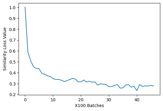
This confirms that we’ve successfully been able to train our network to produce image symbols which are more similar to their corresponding label symbols than was the case with our initial, random parameters. Below, we’ll see if this is a sufficiently useful result to do classification.

Evaluation

To test the network’s generalization performance, we’ll load the set of Fashion-MNIST test data. These are 10,000 images of garments which were not used to train the network:

#load the full set of testing data to evaluate the network
x_test, y_test = tfds.as_numpy(tfds.load(dataset_name, 
                    split=['test'], 
                    data_dir="~/data",
                    shuffle_files=False,
                    as_supervised=True,
                    batch_size=-1,
                    with_info=False))[0]

To produce a class prediction from the network given its set of trained parameters, the symbol the network produces from an image is compared to the set of class symbols. The class symbol the image symbol is most similar to is chosen as its predicted label:

def predict(network, params, x, class_codebook = class_codebook):
    #apply the network given its parameters
    yhat = network.apply(params, x)
    #calculate similarities between the image symbols and label symbols
    similarities = similarity_outer(yhat, class_codebook)
    #return the label the image is most similar to
    classes = jnp.argmax(similarities, axis=1)

    return classes

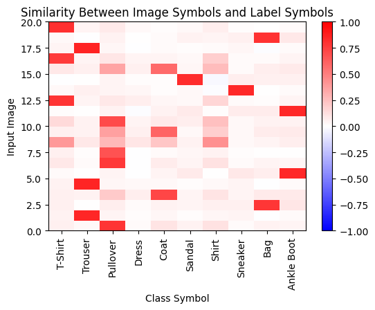
In the image below, each row corresponds to an input image, and each column is a class. The predicted class for each image can be identified by finding the highest similarity value in its row. We can see by this plot that the network has become much better at transforming input images into symbols which are similar to the class labels:

#compute the symbols which the network produces from images
symbols_1 = network.apply(params, images_full[0:batch_size,...])
#show each image symbol's similarity to the class symbols
plot_similarity(symbols_1[0:20,...])

png

To calculate the network’s overall classification accuracy, we simply calculate the average rate its predicted labels match the true labels:

def accuracy(network, params, x, y, class_codebook = class_codebook):
    classes = predict(network, params, x, class_codebook)
    accuracy = jnp.mean(classes == y)

    return accuracy

Our accuracy on the test set is 89%, and accuracy on the original training set is slightly higher at 92%:

test_acc = accuracy(network, params, x_test, y_test).item()
print("Test accuracy is", test_acc)

train_acc = accuracy(network, params, images_full, labels_full)
print("Training accuracy is", train_acc)

Test accuracy is 0.8899999856948853
Training accuracy is 0.91373336

Furthermore, now that images can be transformed into symbols, we can compute with them in the same ways we’ve previously demonstrated: these symbols can be compared against lists and constructed into graphs. For example, let’s compute if a given image belongs to the set of [T-Shirt, Pullover, Shirt]:

clothing_set = bundle_list(tshirt, pullover, shirt)

As we can see, the symbol produced from an image of a pullover is similar to this set:

similarity(symbols_1[0:1,...], clothing_set).item()

0.5237522125244141

But the symbol produced from an image of trousers is not:

similarity(symbols_1[1:2,...], clothing_set).item()

0.08248300105333328

This is a simple demonstration that we can incorporate the symbols produced by a neural network to do the types of vector-symbolic computations we’ve demonstrated previously (e.g. constructing advanced data structures and comparing them directly).

Conclusion

In this tutorial, we’ve demonstrated how a neural network can be used to transform conventional data - in this case, images - into vector-symbols. We accomplished this by creating a network which maps an input image into the same domain as our vector-symbolic architecture. This network was then trained to map each input image into a symbol which was similar to the image’s matching class label.

However, this is far from the only way in which natural data and/or neural networks can be integrated with vector-symbolic architectures. Images can be also be transformed into composite representations of an image or learn the relationships between different symbols. In many ways, the exploration of ways to integrate these two tools - vector-symbolic computations and neural networks - has just begun.

This notebook concludes this 4-part series of tutorials introducing vector-symbolic architectures. To recap this series, we first introduced the basic elements of VSAs: vector-symbols and the similarity metric between them. We then demonstrated vector-symbolic operations: bundling and binding. Finally, we discussed how neural networks can be used to map real-world data into vector-symbols.

For those interested in learning more, recent surveys into VSAs can provide a much more comperehensive explanation of their operations, applications, and challenges. The VSA-Online group also organizes regular talks in ongoing research using VSAs.